
DisCov metric
DisCov, short for Distribution of Coverage, summarises whether coverage across a reference sequence looks broad and well distributed or narrow, patchy, and uneven. This new metric was introduced by Anvi’o team (and in particular Iva Veseli, see this PR).
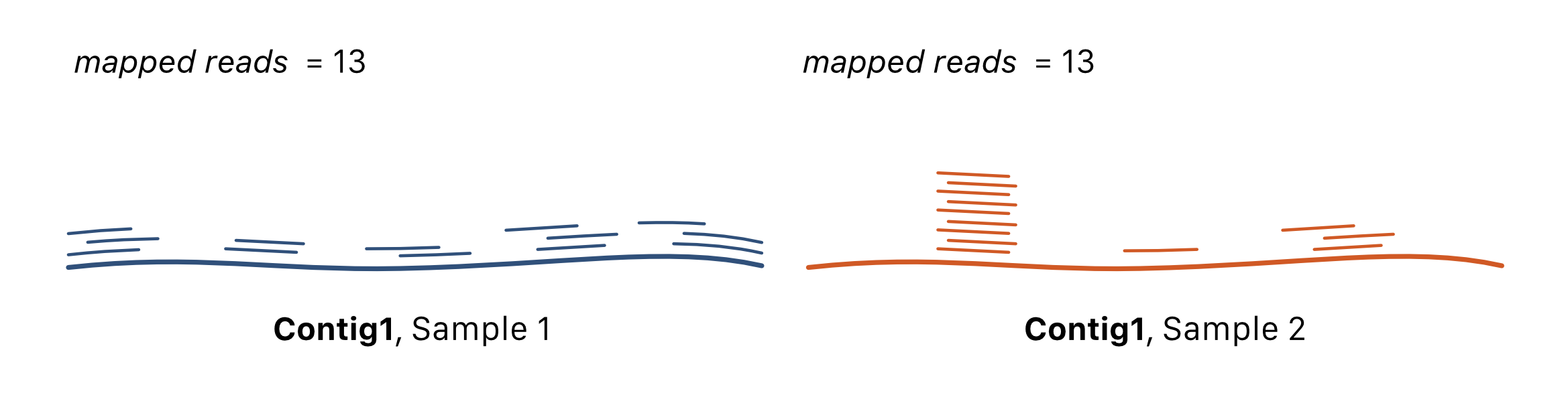
Average coverage is useful, but it can hide important structure, as shown in the figure where 13 reads mapped against the same contig can offer different levels of confidence of the detection of the contig itself (left) or spurious mappings from other sources (right).
DisCov adds two checks that average depth does not answer:
- Spread: how much of the sequence has any coverage?
- Evenness: where coverage exists, is the depth close to the typical nonzero depth?
The final score ranges from 0 to 1. Higher values mean the coverage is both broader and more even.
Components
DisCov is built from two component scores, S and E.
Spread score
The spread score, S, measures how many windows across the sequence have any coverage.
The sequence is split into non-overlapping windows. Each window is counted as covered if at least one base in that window has depth greater than zero.
S = covered_windows / total_windows
For example, if 8 out of 10 windows have coverage:
S = 8 / 10 = 0.8
A high S means coverage is present across most of the sequence. A low S means coverage is concentrated in only a few regions.
Evenness score
The evenness score, E, measures whether covered bases have similar depth.
DisCov first ignores bases with zero coverage, then calculates the median of the remaining nonzero depths. Each covered base is then checked against an acceptable fold range around that median.
With the default range, a base is considered typical if its depth is between 0.5x and 2.0x the median nonzero depth. If the median nonzero depth is 20x, the default acceptable range is:
10x to 40x
The evenness score is:
E = covered_bases_within_range / covered_bases
For example, if 900 out of 1,000 covered bases fall between 10x and 40x:
E = 900 / 1000 = 0.9
A high E means the covered parts of the sequence have consistent depth. A low E means coverage is uneven, with many bases much lower or much higher than the typical covered base.
Score formulas
By default, DisCov combines spread and evenness with the linear formula:
DisCov = alpha * S + (1 - alpha) * E
The alpha parameter controls the weight given to spread.
With the default alpha = 0.5, spread and evenness are weighted equally:
DisCov = 0.5 * S + 0.5 * E
For example, if S = 0.8 and E = 0.9:
DisCov = 0.5 * 0.8 + 0.5 * 0.9 = 0.85
BamCountRefs also supports a geometric formula:
DisCov = S^alpha * E^(1 - alpha)
The geometric formula is stricter when one component is much lower than the other.
Using DisCov
DisCov is available from bamcountrefs:
bamcountrefs --discov input.bam
With --output, BamCountRefs writes a separate table:
bamcountrefs --output results/sample --discov input/*.bam
This creates:
results/sample_discov.tsv
DisCov requires per-base depth tracking, so it uses extra memory proportional to reference length. It is also included by --all-metrics.
The main options are:
| Option | Default | Meaning |
|---|---|---|
--discov-window |
1000 |
Window length used for the spread score |
--discov-fold-lower |
0.5 |
Lower fold bound around the median nonzero depth |
--discov-fold-upper |
2.0 |
Upper fold bound around the median nonzero depth |
--discov-alpha |
0.5 |
Weight assigned to the spread score |
--discov-formula |
linear |
Formula used to combine S and E; either linear or geometric |
Interpreting Scores
DisCov values are easiest to compare when they were calculated with the same parameters.
| DisCov value | Interpretation |
|---|---|
Close to 0 |
Little or no convincing coverage |
Around 0.3 |
Weak or highly patchy coverage |
Around 0.5 |
Ambiguous coverage |
Around 0.7 |
Reasonably convincing coverage |
Close to 1 |
Broad and even coverage |
These are practical guideposts, not universal thresholds. The best cutoff depends on sequencing depth, mapping stringency, reference similarity, and how conservative the analysis needs to be.
Why Average Coverage Is Not Enough
Average coverage answers how much depth exists overall. It does not answer where that depth is.
Consider two references with the same average coverage:
| Scenario | Coverage pattern | Average coverage | Expected DisCov |
|---|---|---|---|
| Broad coverage | Reads are distributed across most windows | Moderate | High |
| Local pileup | Reads cover one small region very deeply | Moderate | Low |
Both references can have the same mean depth, but they should not be interpreted the same way. DisCov helps distinguish broad evidence from localized pileups.
Toy Examples
Suppose a sequence is divided into 10 windows.
Broad and even
Coverage is present in all 10 windows, and depth is fairly similar.
S = 10 / 10 = 1.0E = 0.9- With equal weighting,
DisCov = 0.95
This looks like strong, well-distributed evidence.
Sparse but even
Coverage is present in only 2 out of 10 windows, but those covered regions are internally even.
S = 2 / 10 = 0.2E = 0.9- With equal weighting,
DisCov = 0.55
This is less convincing because most of the sequence has no coverage.
Broad but uneven
Coverage is present in 9 out of 10 windows, but depth varies strongly.
S = 9 / 10 = 0.9E = 0.4- With equal weighting,
DisCov = 0.65
This suggests broad coverage, but the uneven depth may point to mixed signals, repeats, strain variation, mapping artifacts, or other biological or technical complications.
Parameter Choices
The window size controls how finely the sequence is divided.
Smaller windows make S more sensitive to local gaps. Larger windows smooth over small uncovered regions.
If a sequence is shorter than the requested window size, the whole sequence is treated as one window. For longer sequences, tiny trailing windows smaller than 10% of the requested window size are ignored so that a very short final fragment does not dominate the spread score.
The fold range controls how strict the evenness score is. A narrow range makes E more sensitive to coverage variation.
The median nonzero depth is used because it is less sensitive to extreme pileups than the mean.
Edge Cases
If there is no coverage anywhere, all components are zero:
S = 0
E = 0
DisCov = 0
For very short contigs, the spread score can be coarse because there may be only one window.
In those cases, a small amount of coverage can give S = 1, so the score should be interpreted with extra care.